library(ggplot2) # loads the ggplot2 package, assuming you have it installed.
library(ggsoccer) # loads the ggsoccer package
library(dbplyr) # loads the dbplyr package5 RStudio Interface - Practical
5.1 Introduction
Note: This practical assumes that you have R and RStudio installed on your computer. If not, you’ll need to do this first before proceeding.
The pre-class reading for this section covered a number of topics, which we’ll revise today:
The RStudio Interface
Installing and Loading Packages
Project Management in RStudio
5.2 The RStudio Interface
Demonstration
Console
The Console window is where you see the commands that have been executed in R.
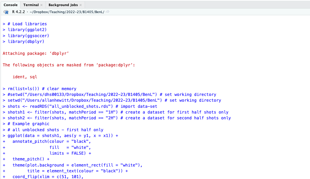
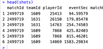
You can type commands directly into the Console, for example here I have entered the command head(shots):
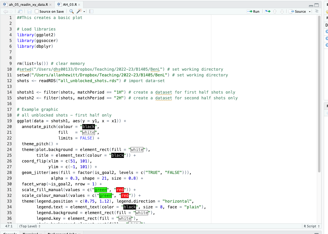
Script editor
Rather than typing commands directly into the Console window, you can write scripts in the Script Editor. You can run full scripts from here, or work through scripts in sections. You can also save and load scripts, and you can call other scripts from within your script.
It’s likely that you will spend most of your time using the Script editor.
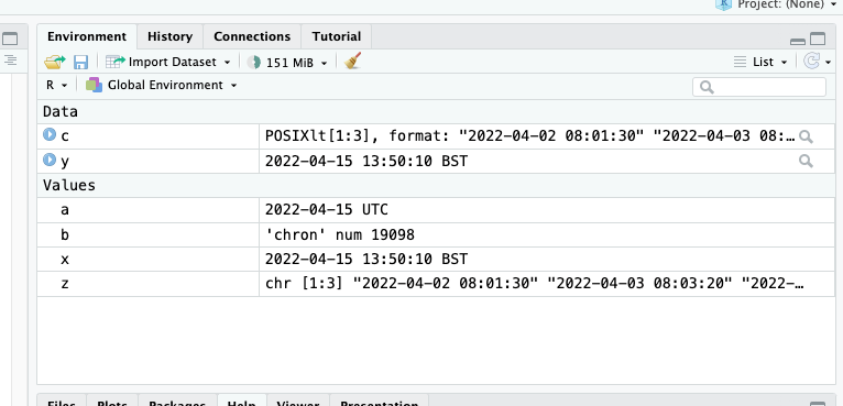
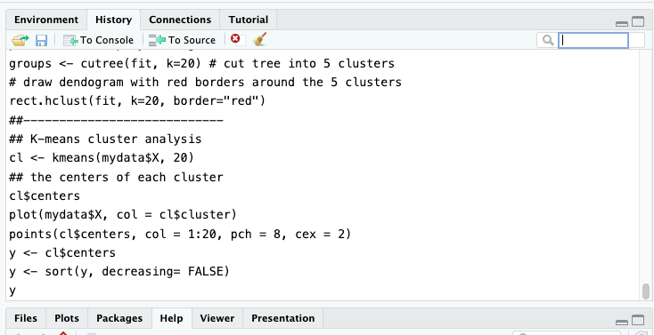
Environment
The Environment window allows you to view variables, data, and functions in the current workspace:
History
The History window allows you to access previously executed commands:
Plots
Any plots you create are presented in the Plots window:
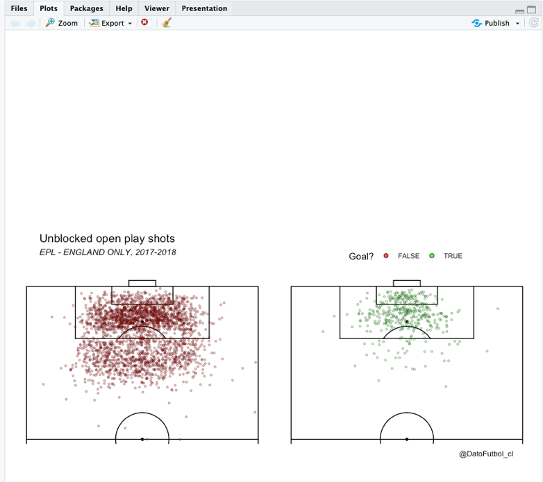
All your plots are stored here, and you can easily save and/or export plots from this window.
5.3 Installing and Loading Packages
Demonstration
When you load RStudio (or R), you automatically load the ‘base’ package. This lets you do lots of things, but we often want to take advantage of the many additional packages that have been created to extend R’s functionality.
Tip
One of the issues you may run into when working with someone else’s R code is that they have used a package that you don’t have installed locally. It’s always worth checking what packages they’ve used, by looking at the first few lines of each script.
First, you need to download and install the package you wish to use. You only need to do this once on each computer you are using.
Go to Tools -> Install Packages.
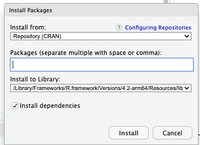
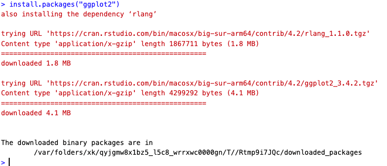
Type the name of the package you wish to install. Here, I’m going to install a package called ‘ggplot2’.
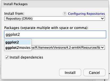
Now, click ‘install’ and the package will install to your computer. Remember, you only have to do this once on each computer you use. You do need to load the library each time you use it (see below).
Now, each time you wish to use the package, you need to load it. The easiest way to do this is to use the ‘library’ command at the start of your script. For example, these three lines of code load three packages (‘ggplot2’, ‘ggsoccer’, ‘dbplyr’). Those packages are then available to you. If you don’t have them installed, you’ll need to download them first.
Also note that, in the code above, the hash sign ‘#’ is used in R to indicate a comment, rather than a line of code to be executed.
You need to put a hash at the start of every line you wish to comment.
Help when using packages
R’s in-built documentation is incredibly helpful for understanding what a specific function does, its inputs, outputs, and potential caveats. To access the documentation for a particular function in R, you can use the help() function or simply type ?.
Example:
# Access documentation for the "mean" function
help(mean)  # or you can use ?mean
You can also use the help() function to get information on datasets in R (note that R comes with a number of existing datasets built-in, which you can use to practice on).
# Access documentation for the "mtcars" dataset
help(mtcars)
Exercise 1: Access and review the documentation for the median() function.
The documentation for each R function typically consists of the following sections:
- Description: A brief overview of what the function does.
- Usage: How the function is used, including the necessary parameters.
- Arguments: Detailed description of the function’s arguments.
- Details: More specific information about the function’s behavior.
- Value: The output of the function.
- See Also: Links to related functions.
- Examples: Some working code examples demonstrating the function’s use.
Show solution
help(median)Exercise 2: Access and review the documentation for the plot() function, and interpret the output.
Show solution
help(plot)Exercise 3: Install and load the dplyr package, then access its documentation.
Show solution
# Check if dplyr is installed
if (!require(dplyr)) {
    # If ggplot2 is not installed, install it
    install.packages("dplyr")

    # Load the dplyr package after installation
    library(dplyr)
} else {
    # If dplyr is already installed, just load it
    library(dplyr)
}
Some packages come with vignettes - detailed documents providing a comprehensive overview of the package, including illustrative examples. You can access vignettes using the vignette() function.
# List all vignettes for 'dplyr' package
vignette(package="dplyr")
To access a specific vignette, just provide its name:
# Access the 'rowwise' vignette from the dplyr package
vignette("rowwise", package = "dplyr")
Exercise 4: Load the ‘grouping’ vignette for the dplyr package.
Show code
vignette("grouping", package = "dplyr")5.4 Project Management in RStudio
You are likely to create a large number of R scripts and files during your MSc SDA programme. It can sometimes be tricky to keep track of everything, especially if you wish to return to something at a later date.
Therefore, I recommend that you create a new R Project for each analysis or tutorial you conduct.
Creating separate RStudio projects for each new work has a number advantages:
Isolation: Each project operates independently of others. This means that workspace variables, loaded packages, and options are specific to each project, reducing the chance of conflicts between different works.
Reproducibility: By keeping the data, code, and outputs for a project in one place, it’s easier for others (or your future self) to reproduce your work. You dissertation advisor, for example, may wish to look at your analysis.
Organisation: Separate projects help keep your work organized. Each project is stored in its own directory, making it easier to manage files and resources related to the project.